MMM Quickstart Guide

Welcome to PyMC-Marketing! This library provides powerful Bayesian modeling tools for marketing analytics. PyMC-Marketing is built on top of PyMC, a probabilistic programming library that enables Bayesian inferenc. In this quickstart, we’ll walk through fitting a basic Media Mix Model (MMM) in PyMC-Marketing.

What is Media Mix Modeling?

Media Mix Modeling (MMM) helps marketers understand how different advertising channels contribute to business outcomes (like sales or conversions). MMM answers key questions:

• Which channels drive the most sales?

• What is the Return on Ad Spend (ROAS) for each channel?

• How should I allocate my marketing budget?

Key Concepts

MMM accounts for two important phenomena in advertising:

1. Adstock (Carry-over effect): The impact of advertising doesn’t happen instantaneously—it builds up over time and gradually decays.

2. Saturation: Returns diminish as you increase spend—the first dollar spent is more effective than the millionth dollar.

Let’s see how we can fit a basic MMM model to understand these effects and measure channel contributions.

Note

The focus of PyMC-Marketing is to provide tooling for real application. Typically, we need to think about the causal structure, lift test calibration and advanced budget optimization. This example should be seen as a first step to a more complex and rich tool-box to drive marketing decisions of the order of millions of dollars. In our example gallery, you will find extensive resources to help you and guide you through the MMM modeling iterative process.

Tip

• For an extended version of this example, see MMM Example Notebook. Here we delve deeper into the data generating process and model diagnostics. We also include ROAS estimation and out of sample predictions.

• If you want to see a complete end-to-end analysis, see MMM End-to-End Case Study. Here we take a “real” world dataset and go through the entire process of model specification, fitting, optimization and scenario planning.

Prepare Notebook

Let’s import the necessary libraries:

import arviz as az
import matplotlib.pyplot as plt
import numpy as np
import pandas as pd
from pymc_extras.prior import Prior

from pymc_marketing.mmm import MMM, GeometricAdstock, LogisticSaturation

az.style.use("arviz-darkgrid")
plt.rcParams["figure.figsize"] = [12, 7]
plt.rcParams["figure.dpi"] = 100

%config InlineBackend.figure_format = "retina"

%load_ext autoreload
%autoreload 2

# Set random seed for reproducibility
seed = sum(map(ord, "mmm"))
rng = np.random.default_rng(seed=seed)

Load Data

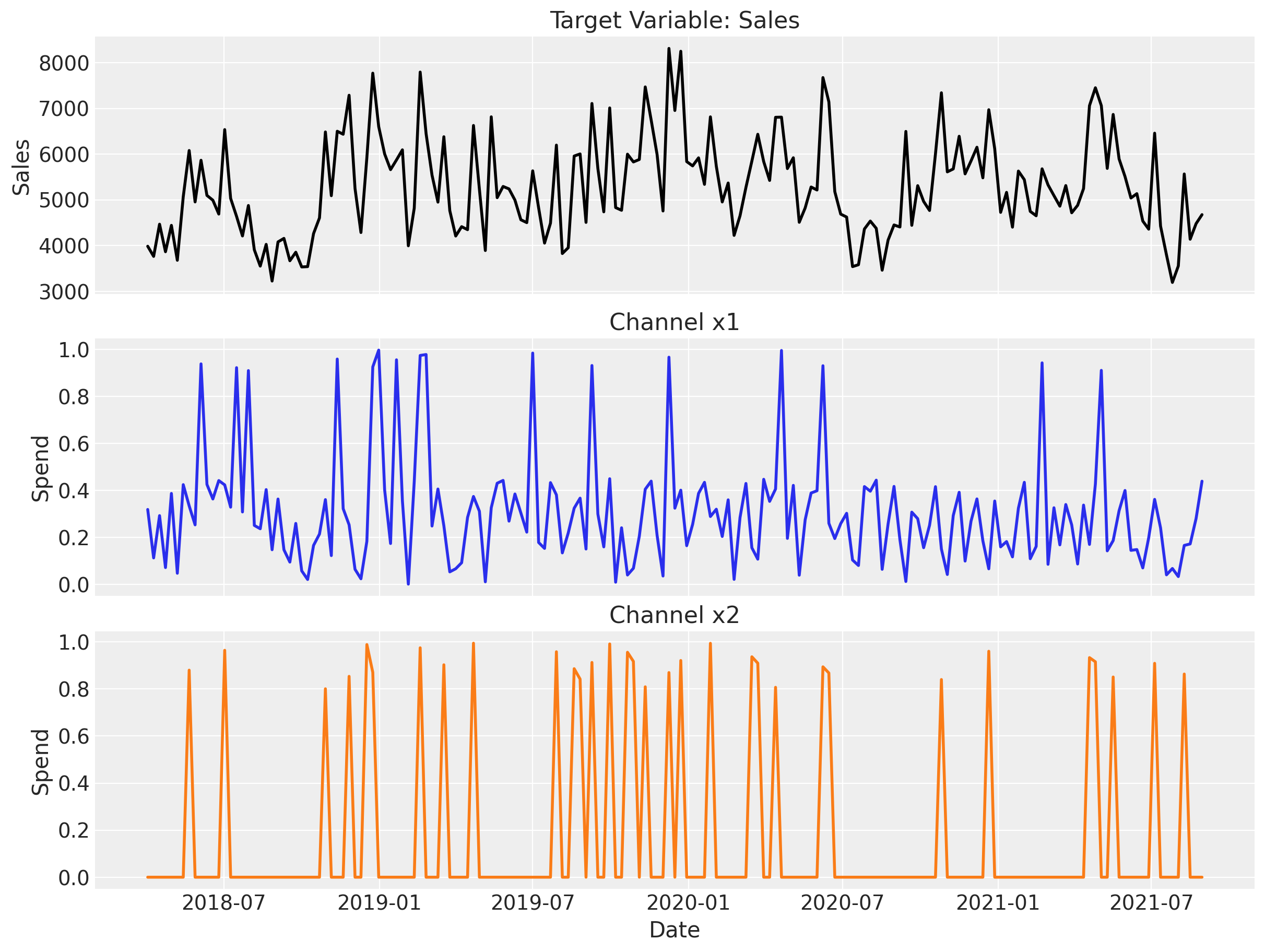
We’ll use a synthetic dataset that simulates weekly sales data along with spend on two marketing channels (x1 and x2), plus some control variables for special events.

# Load the data
url = "https://raw.githubusercontent.com/pymc-labs/pymc-marketing/main/data/mmm_example.csv"
data = pd.read_csv(url, parse_dates=["date_week"])

print(f"Data shape: {data.shape}")
data.head()

Data shape: (179, 8)

	date_week	y	x1	x2	event_1	event_2	dayofyear	t
0	2018-04-02	3984.662237	0.318580	0.0	0.0	0.0	92	0
1	2018-04-09	3762.871794	0.112388	0.0	0.0	0.0	99	1
2	2018-04-16	4466.967388	0.292400	0.0	0.0	0.0	106	2
3	2018-04-23	3864.219373	0.071399	0.0	0.0	0.0	113	3
4	2018-04-30	4441.625278	0.386745	0.0	0.0	0.0	120	4

Let’s visualize our target variable (sales) and the media spend over time:

fig, axes = plt.subplots(3, 1, figsize=(12, 9), sharex=True)

# Sales
axes[0].plot(data["date_week"], data["y"], color="black", linewidth=2)
axes[0].set(ylabel="Sales", title="Target Variable: Sales")

# Channel 1
axes[1].plot(data["date_week"], data["x1"], color="C0", linewidth=2)
axes[1].set(ylabel="Spend", title="Channel x1")

# Channel 2
axes[2].plot(data["date_week"], data["x2"], color="C1", linewidth=2)
axes[2].set(xlabel="Date", ylabel="Spend", title="Channel x2");

Feature Engineering

For our MMM model, we’ll include:

• Trend: A linear trend to capture long-term growth

• Seasonality: Yearly seasonality (handled automatically by the model)

• Events: Binary indicators for special events

• Media channels: Our two advertising channels

# Add a simple linear trend feature
data["t"] = range(len(data))

# Split into features (X) and target (y)
X = data.drop("y", axis=1)
y = data["y"]

print(f"Features: {X.columns.tolist()}")

Features: ['date_week', 'x1', 'x2', 'event_1', 'event_2', 'dayofyear', 't']

Model Specification

Now we’ll configure our MMM model. The key components are:

• Adstock transformation: We use GeometricAdstock with a maximum lag of 8 weeks

• Saturation transformation: We use LogisticSaturation to capture diminishing returns

• Priors: We can customize priors based on domain knowledge

Setting Priors

One powerful feature of Bayesian modeling is the ability to incorporate prior knowledge. Here’s a simple heuristic for channel priors based on spend share:

# Calculate spend share for each channel
total_spend_per_channel = data[["x1", "x2"]].sum(axis=0)
spend_share = total_spend_per_channel / total_spend_per_channel.sum()

print("Spend share per channel:")
print(spend_share)

# Use spend share to inform prior on channel contributions
n_channels = 2
prior_sigma = n_channels * spend_share.to_numpy()

print(f"\nPrior sigma for channels: {prior_sigma}")

Spend share per channel:
x1    0.65632
x2    0.34368
dtype: float64

Prior sigma for channels: [1.31263903 0.68736097]

Now let’s define our model configuration:

my_model_config = {
    "intercept": Prior("Normal", mu=0.5, sigma=0.2),
    "saturation_beta": Prior("HalfNormal", sigma=prior_sigma),
    "gamma_control": Prior("Normal", mu=0, sigma=0.05),
    "gamma_fourier": Prior("Laplace", mu=0, b=0.2),
    "likelihood": Prior("Normal", sigma=Prior("HalfNormal", sigma=6)),
}

# Sampler configuration
my_sampler_config = {"progressbar": True}

# Initialize the MMM model
mmm = MMM(
    model_config=my_model_config,
    sampler_config=my_sampler_config,
    date_column="date_week",
    adstock=GeometricAdstock(l_max=8),
    saturation=LogisticSaturation(),
    channel_columns=["x1", "x2"],
    control_columns=["event_1", "event_2", "t"],
    yearly_seasonality=2,
)

Prior Predictive Check

Tip

The prior predictive check is a good way to check that our priors are reasonable. Hence, is strongly recommended to perform this check before fitting the model. If you are new to Bayesian modeling, take a look into our Prior Predictive Modeling guide notebook.

Before fitting, let’s check that our priors are reasonable:

# Generate prior predictive samples
mmm.sample_prior_predictive(X, y, samples=1_000, random_seed=rng)

# Plot prior predictive distribution
fig, ax = plt.subplots(figsize=(12, 6))
mmm.plot_prior_predictive(ax=ax, original_scale=True)
ax.legend(loc="upper left")
ax.set_title("Prior Predictive Check");

Sampling: [adstock_alpha, gamma_control, gamma_fourier, intercept, saturation_beta, saturation_lam, y, y_sigma]

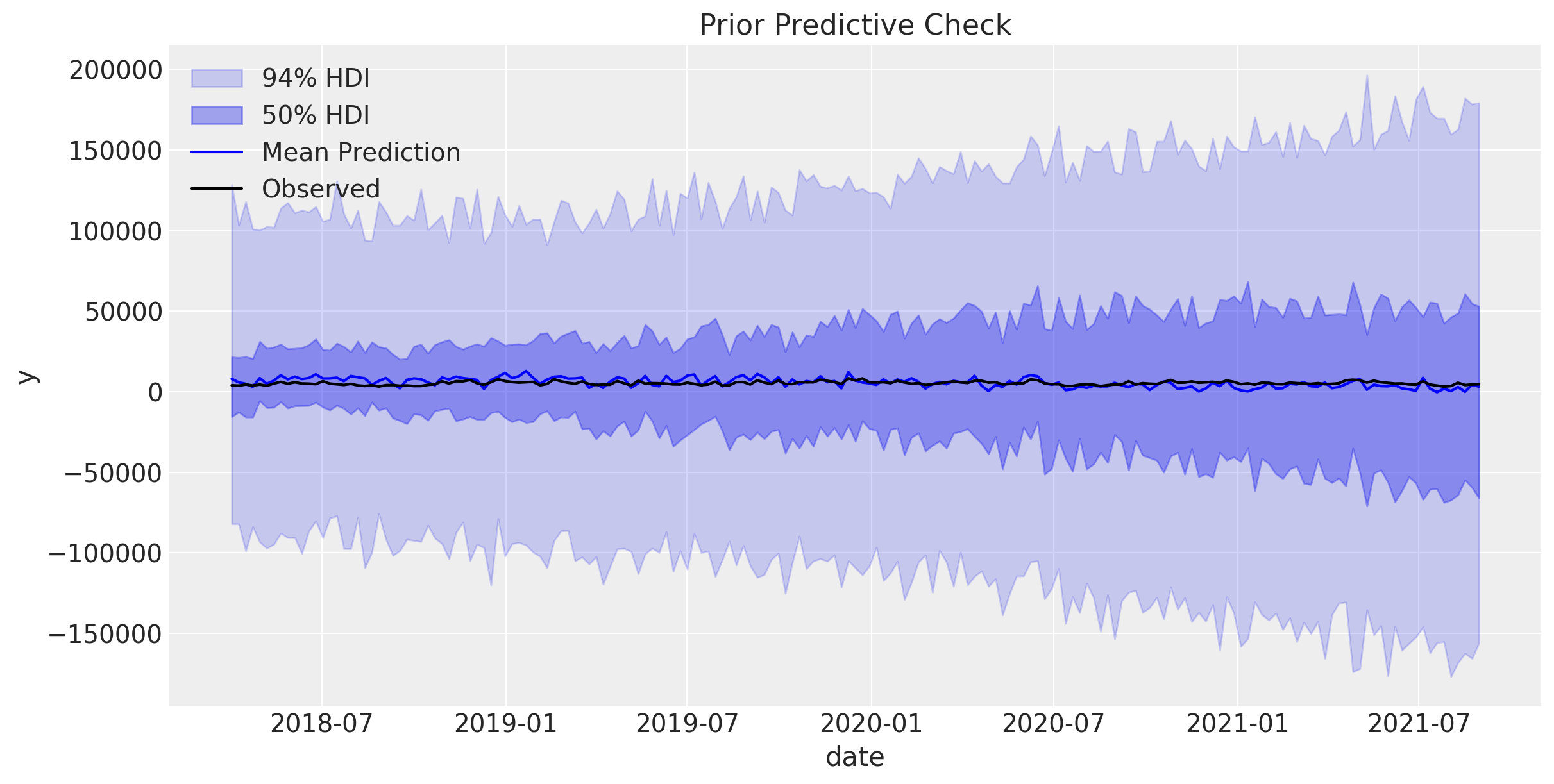
Overall, the prior predictive check looks good.

Model Fitting

Now let’s fit the model to our data using MCMC sampling. Observe that we can use different samplers by passing the nuts_sampler argument. For instance, we can use numpyro nutpie or blackjax samplers (see Other NUTS Samplers for more details).

# Fit the model
_ = mmm.fit(
    X=X,
    y=y,
    chains=4,
    target_accept=0.85,
    nuts_sampler="numpyro",
    random_seed=rng,
)

Model Diagnostics

After fitting, we should check the model quality. Let’s start with divergences:

# Check for divergences
n_divergences = mmm.idata["sample_stats"]["diverging"].sum().item()
print(f"Number of divergences: {n_divergences}")

if n_divergences == 0:
    print("✓ No divergences - sampling was successful!")
else:
    print("⚠ Warning: Model had divergences. Consider increasing target_accept.")

Number of divergences: 0
✓ No divergences - sampling was successful!

Parameter Summary

Let’s examine the estimated parameters:

# Plot traces for key parameters
_ = az.plot_trace(
    data=mmm.fit_result,
    var_names=[
        "saturation_beta",
        "saturation_lam",
        "adstock_alpha",
    ],
    compact=True,
    backend_kwargs={"figsize": (10, 6), "layout": "constrained"},
)
plt.gcf().suptitle("Trace Plots", fontsize=16);

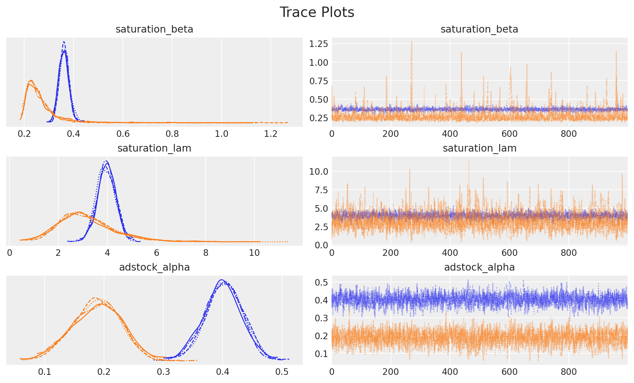
Good trace plots should show:

• Left side: Smooth, bell-shaped distributions

• Right side: “Fuzzy caterpillar” patterns (good mixing) with no trends

Posterior Predictive Check

How well does our model fit the observed data?

# Sample from posterior predictive distribution
mmm.sample_posterior_predictive(X, extend_idata=True, combined=True)

# Plot model fit
fig = mmm.plot_posterior_predictive(original_scale=True)

Sampling: [y]

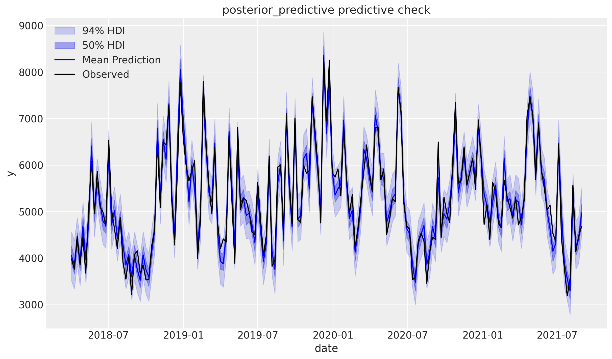
The model captures the observed data well if the black dots (actual sales) fall within the shaded uncertainty bands.

Contribution Analysis

Now for the fun part—understanding how much each component contributes to sales!

Component Contributions Over Time

Let’s visualize the contribution of each component of the model over time:

fig = mmm.plot_components_contributions(original_scale=True)
plt.suptitle("Component Contributions to Sales", fontsize=16, y=1.02);

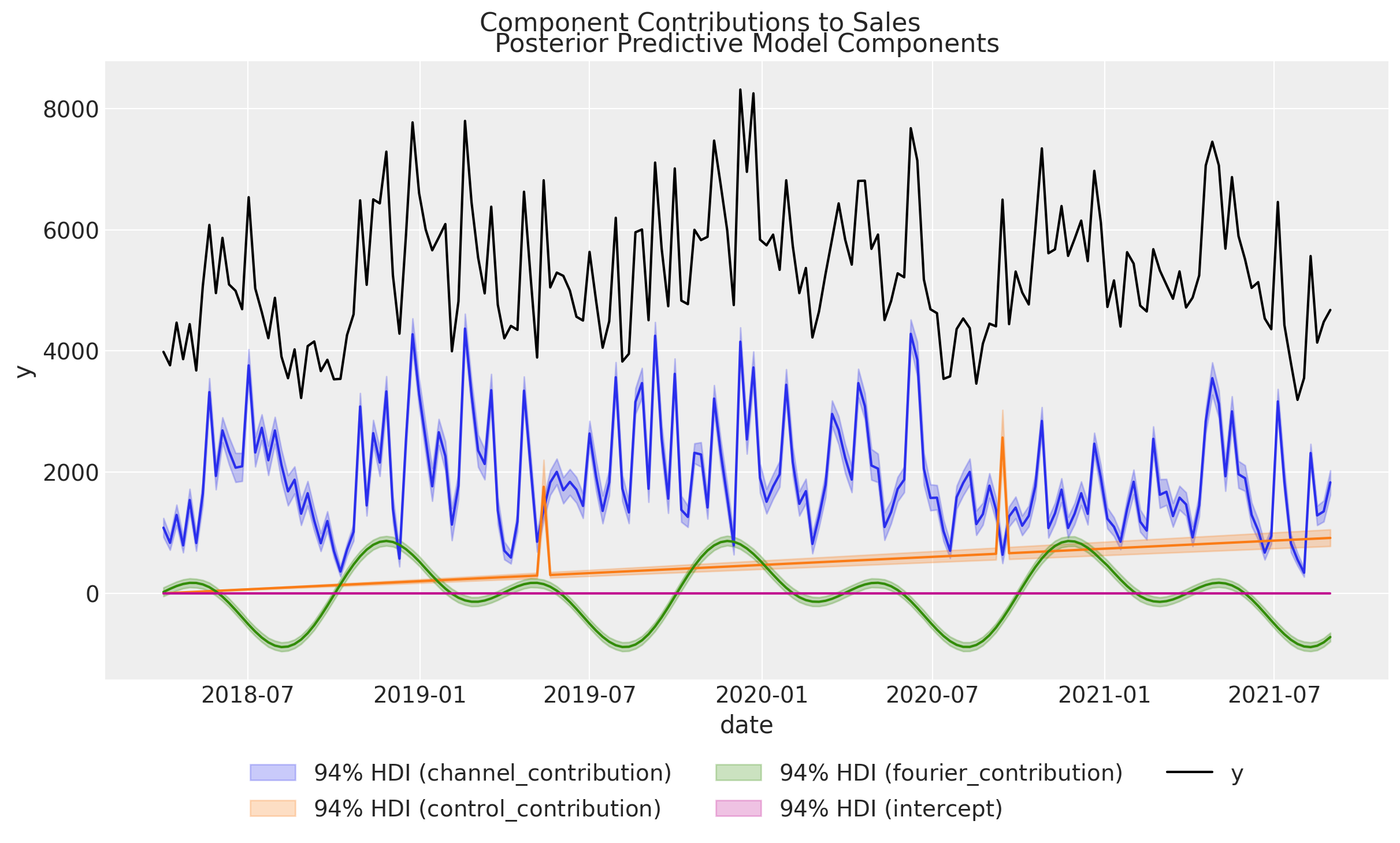
We see that we have captured the linear trend, events contributions and the seasonalities in the data. The remaining variation is due to the media channels, which is exactly what we want to understand.

Waterfall Chart: Total Contribution by Component

A waterfall chart shows the total contribution of each component across the entire time period:

# Waterfall decomposition
fig = mmm.plot_waterfall_components_decomposition();

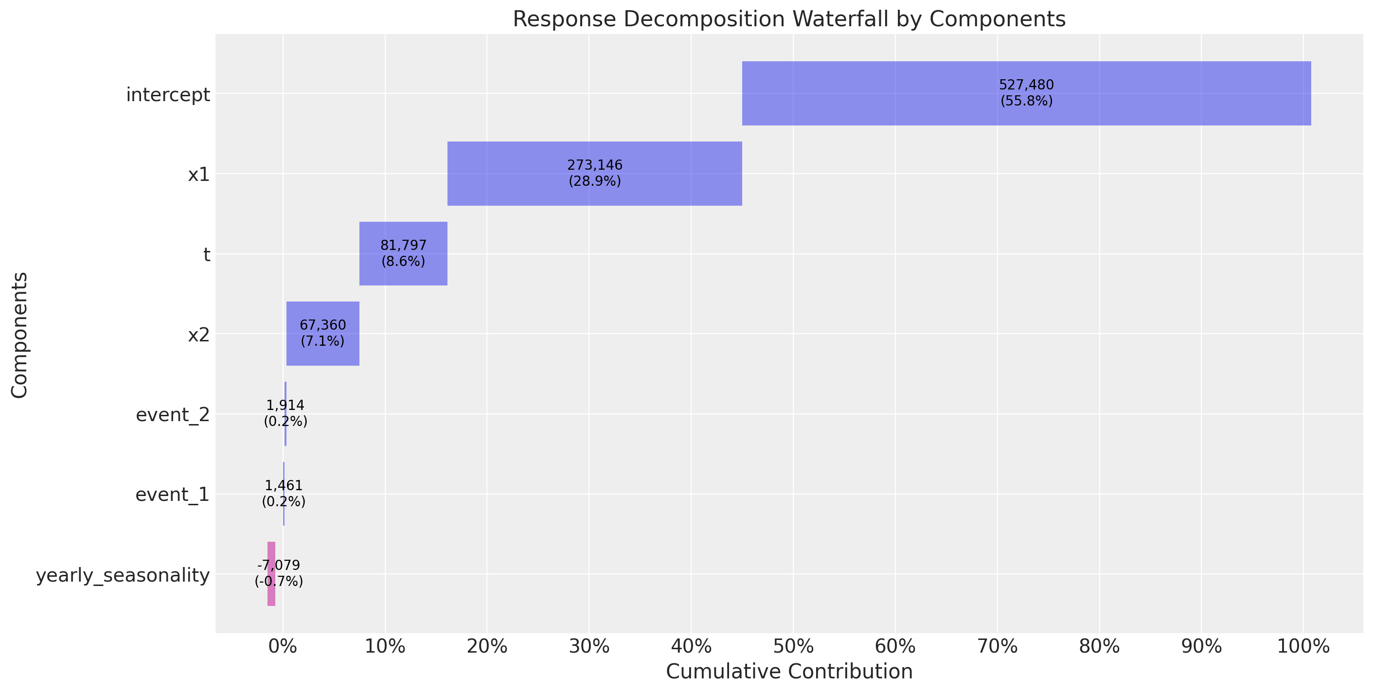
This chart answers the question: “How much did each component contribute to total sales?”

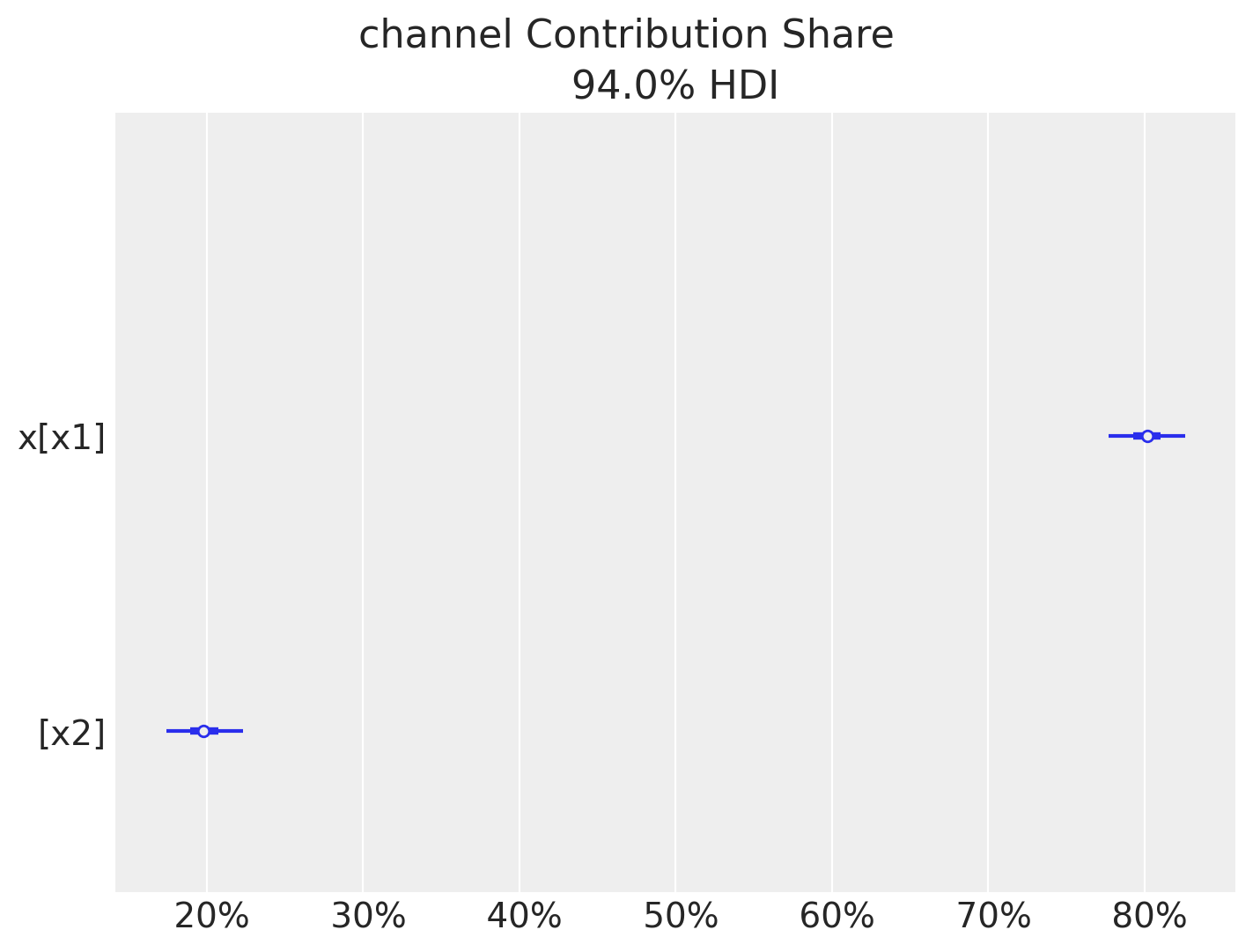
Channel Contribution Share

What percentage of media-driven sales comes from each channel?

# Plot channel contribution share
fig = mmm.plot_channel_contribution_share_hdi(figsize=(7, 5));

Direct Contribution Curves

These curves show the relationship between spend and contribution, accounting for saturation:

# Plot direct contribution curves (saturation curves)
fig = mmm.plot_direct_contribution_curves()
plt.suptitle("Direct Contribution Curves", fontsize=16, y=1.02);

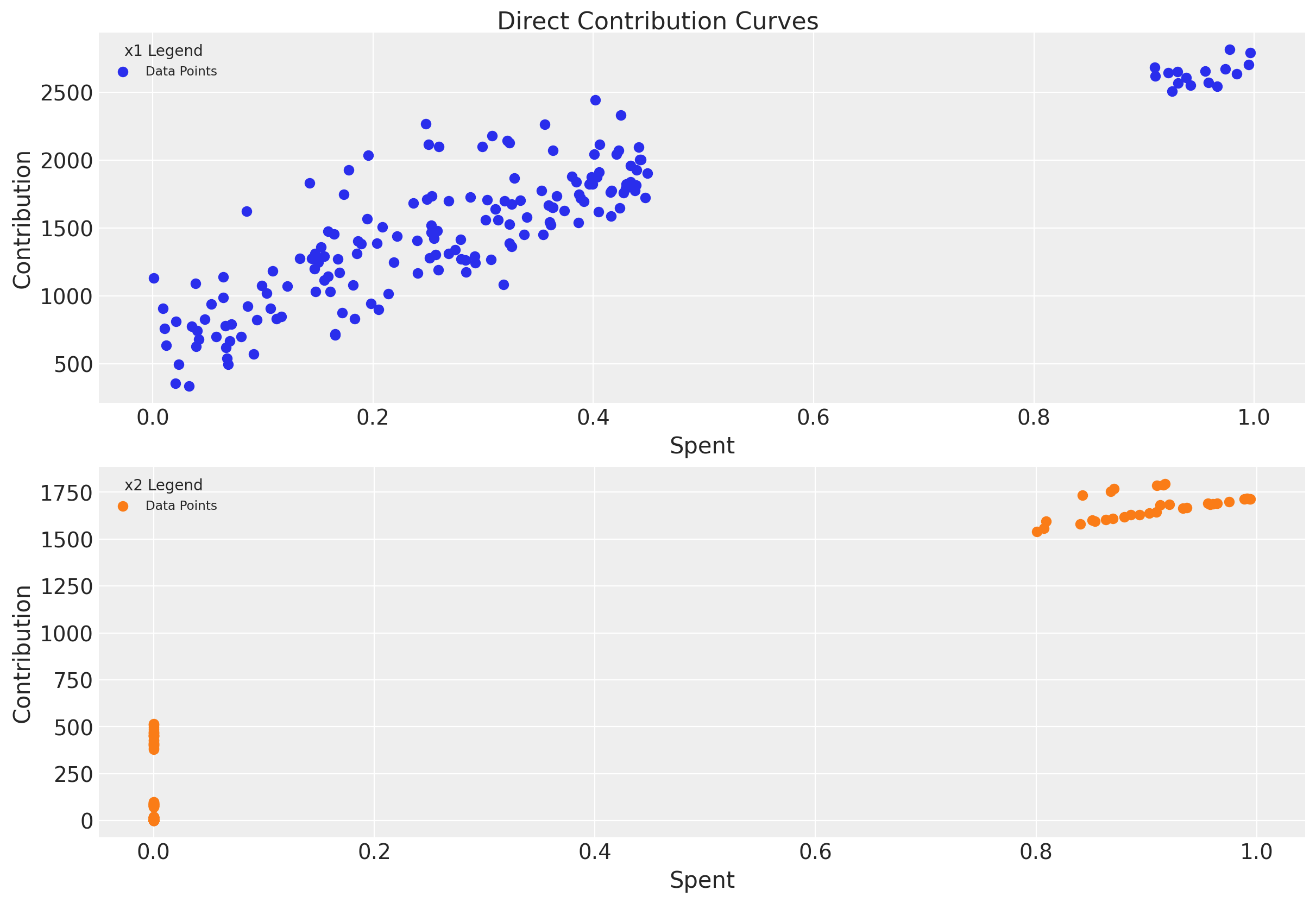
Notice how the curves flatten at higher spend levels—this is the saturation effect in action!

Channel Contribution Grid

A complementary view of the media performance is to evaluate the channel contribution at different share spend levels for the complete training period. Concretely, if we denote by \(\delta\) the input channel data percentage level, so that for \(\delta = 1\) we have the model input spend data and for \(\delta = 1.5\) we have a \(50\%\) increase in the spend, then we can compute the channel contribution at a grid of \(\delta\)-values and plot the results:

mmm.plot_channel_contribution_grid(start=0, stop=1.5, num=12, absolute_xrange=True);

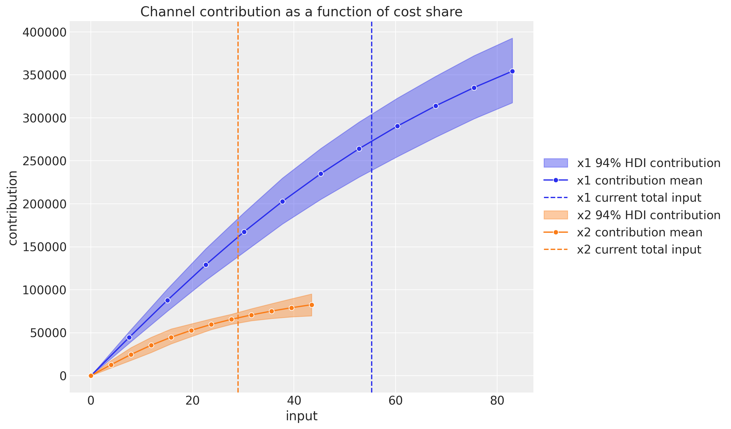
Here we can also see the saturation effect and the relative contribution of each channel as a function of the share spend level on the aggregate time period.

Next Steps

Congratulations! You’ve successfully fitted your first MMM model with PyMC-Marketing. 🎉

To continue your journey, check out:

• MMM Example Notebook: A comprehensive walkthrough including data generation, ROAS calculation, and more advanced diagnostics

• Budget Allocation with PyMC-Marketing: Learn how to optimize your marketing budget allocation

• Lift Test Calibration: Incorporate experimental results to improve model accuracy

• MMM with time-varying parameters (TVP): Model changing baseline effects over time

• MMM with time-varying media baseline: Model changing media efficiency over time

PyMC-Marketing MMM Features

PyMC-Marketing provides a comprehensive suite of tools for Marketing Mix Modeling:

Feature	Description
Custom Priors and Likelihoods	Tailor your model to your specific business needs by including domain knowledge via prior distributions
Adstock Transformation	Optimize the carry-over effects in your marketing channels
Saturation Effects	Understand the diminishing returns in media investments
Customize adstock and saturation functions	Select from a variety of adstock and saturation functions, or implement your own custom functions
Time-varying Intercept	Capture time-varying baseline contributions using modern and efficient Gaussian processes approximation methods
Time-varying Media Contribution	Capture time-varying media efficiency in your model
Visualization and Model Diagnostics	Get a comprehensive view of your model’s performance and insights
Causal Identification	Input a business-driven directed acyclic graph to identify meaningful variables for causal conclusions
Multiple inference algorithms	Choose between various NUTS samplers (e.g., BlackJax, NumPyro, and Nutpie)
GPU Support	PyMC’s multiple backends allow for GPU acceleration
Out-of-sample Predictions	Forecast future marketing performance with credible intervals for simulations and scenario planning
Budget Optimization	Allocate your marketing spend efficiently across various channels for maximum ROI
Experiment Calibration	Fine-tune your model based on empirical experiments (lift tests) for a more unified view of marketing

References

• Jin, Y., Wang, Y., Sun, Y., Chan, D., & Koehler, J. (2017). Bayesian Methods for Media Mix Modeling with Carryover and Shape Effects.

• PyMC-Marketing Documentation

• Juan Orduz, Media Effect Estimation with PyMC: Adstock, Saturation & Diminishing Returns

%load_ext watermark
%watermark -n -u -v -iv -w -p pymc_marketing

Last updated: Sun Oct 05 2025

Python implementation: CPython
Python version       : 3.12.11
IPython version      : 9.3.0

pymc_marketing: 0.15.1

pymc_extras   : 0.4.0
numpy         : 2.2.0
pymc_marketing: 0.15.1
matplotlib    : 3.10.3
arviz         : 0.21.0
pandas        : 2.3.0

Watermark: 2.5.0